Matlab da Sinyal İşleme

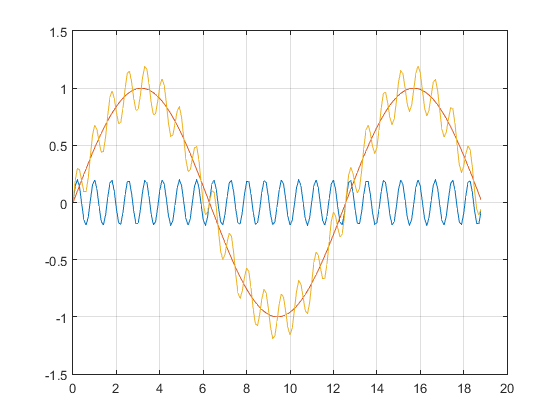
t = 0:0.1:6*pi; % X düzleminde aralağımız
A = 0.2; % Dalgalanma şiddeti
y1 = A * sin(t * 8); % İlk sinusoid
y2 = sin(t/2); % İkinci sinusoid

%plot(t, y1)
%grid on % Çizilen verilerin anlaşılabilirliği için grid i açar

%subplot(2,1,2) % bu kod parçaçığı aynı ekranda iki tane çıktı göstermemizi sağlar
%plot(t, y1, t, y2)
%grid on % Çizilen verilerin anlaşılabilirliği için grid i açar

y3 = y1 + y2; % iki sinus sinyalinin birleştirilmesi

plot(t, y1, t, y2, t, y3)
%subplot(2,1,2)
%plot(t,y3) % birleştirlen sinus sinyallerinin çizilmesi
grid on % Çizilen verilerin anlaşılabilirliği için grid i açar

Grafik İşlemleri-1

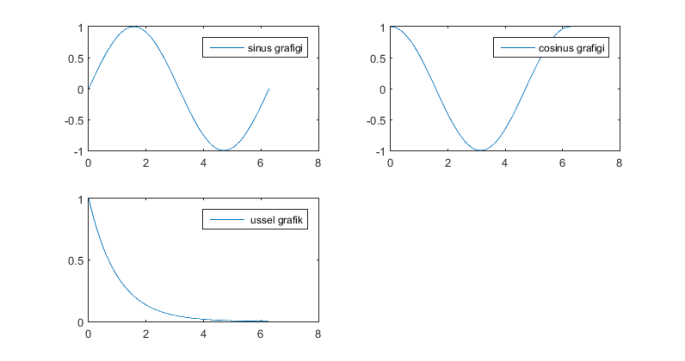
x=0:pi/100:2*pi;
y1=sin(x);
y2= cos (x);
y3= exp (-x);
subplot (2,2,1);
plot (x,y1);
legend (‘sinus grafigi’);
subplot (2,2,2);
plot (x,y2);
legend(‘cosinus grafigi’);
subplot (2,2,3);
plot (x,y3);
legend (‘ ussel grafik ‘);

Grafik İşlemleri-2

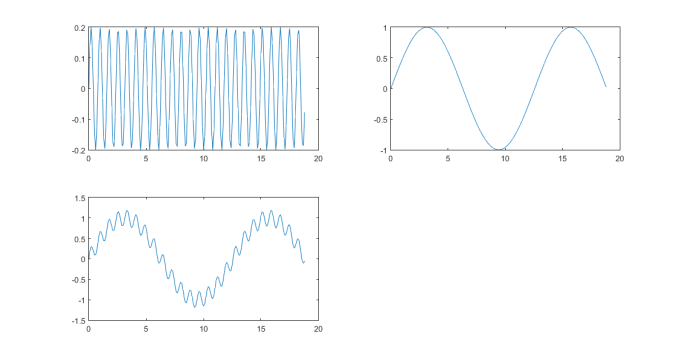
t = 0:0.1:6*pi; % X düzleminde aralağımız
A = 0.2; % Dalgalanma şiddeti
y1 = A * sin(t * 8); % İlk sinusoid
y2 = sin(t/2); % İkinci sinusoid
y3 = y1 + y2; % iki sinus sinyalinin birleştirilmesi

subplot (2,2,1);
plot (t, y1)

subplot (2,2,2);
plot (t, y2)

subplot (2,2,3);
plot (t, y3)

Grafik İşlemleri-3

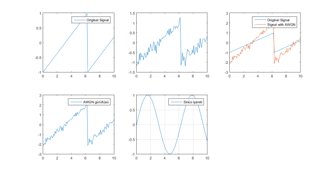
t = (0:0.1:10)’;
x = sawtooth(t);
y = awgn(x,10,’measured’);

y2 = x + y % işaret ile gürültünün toplanılması

subplot (2,3,1);
plot(t,x)
legend(‘Original Signal’)

subplot (2,3,2);
plot(t,y)

subplot (2,3,3);
plot(t,[x,y2])
legend(‘Original Signal’,’Signal with AWGN’)

subplot (2,3,4);
plot(t,y2)
legend(‘AWGN gürültüsü’)

subplot (2,3,5);
plot(t,sin(t)), grid on
legend (‘Sinüs işareti’)

Grafik İşlemleri-4